Quickstart

This notebook demonstrates how to use pcxarray to query and prepare a time series of HLS data that is suitable for monitoring water turbidity trends in the Mississippi Sound.

First - defining a region of interest

A geometry denoting the region of interest (ROI) is required to both query against the Planetary Computer data catalog and to facilitate the preparation of the imagery. The CRS of the geometry is important, as all results from ``pcxarray`` will be returned in the same CRS as the geometry (and reprojected if necessary). By default, pcxarray assumes any geometry it receives for any query or preparation operation is in WGS84 (EPSG:4326). Naturally, using a geographic CRS is often suboptimal for most applications, so it is highly recommended to transform a given ROI geometry to an appropriate projected CRS before using it with pcxarray.

In this example, a rectangular geometry over the Mississippi Sound region in the northern Gulf Coast of the United States is used. Once the geometry is defined, it will be added to a GeoPandas GeoDataFrame, which will enable quick and easy projection to UTM 16N and visualization of the ROI later. Technically, a GeoDataFrame is not required, but it makes certain reprojection and plotting tasks easier.

NOTE: While the geometry is technically horizontal in its native Geographic CRS, it will be angled slightly in the projected CRS. Applying ``.envelope`` on the geometry will return another rectangular geometry that encompasses the original geometry without any rotation in the projected CRS. Usage of this envelope geometry is not required, but is used in this example to prevent the ROI from appearing rotated in the projected CRS.

from shapely.geometry import Polygon
import geopandas as gpd

utm_16n_crs = "EPSG:32616"  # UTM Zone 16N

geom = Polygon([
    [-89.66184148070946, 30.43851678975875],
    [-89.66184148070946, 30.10426503400744],
    [-87.67251376704150, 30.10426503400744],
    [-87.67251376704150, 30.43851678975875],
    [-89.66184148070946, 30.43851678975875]
])
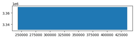
ms_sound_gdf = gpd.GeoDataFrame({"geometry": [geom]}, crs="EPSG:4326")
ms_sound_gdf = ms_sound_gdf.to_crs(utm_16n_crs)  # UTM 16N
ms_sound_gdf["geometry"] = ms_sound_gdf["geometry"].envelope  # Get the envelope to avoid rotation in UTM
ms_sound_gdf.plot()

roi_geom = ms_sound_gdf["geometry"].values[0]

Now that the geometry is defined, it can be used to query the Planetary Computer data catalog for HLS imagery. In order to query using pcxarray, in addition to the geometry, the name of the collection to query against is required. The collection IDs can be found in the Planetary Computer data catalog website, or by using the get_pc_collections function from pcxarray. This function returns a GeoDataFrame of all collections available in the Planetary Computer data catalog and their spatial extents, which can be helpful when searching for a specific collection.

In Planetary Computer, HLS data is divided into two collections: one for Landsat data and one for Sentinel-2 data. This is not the norm, however, because the bands provided in the two collections are different, they are intentionally kept separate. Data from both collections can be used as part of the same processing pipeline, but it is good to be aware of the differences in the bands provided in each collection. See the Planetary Computer page on HLS v2.0 for more details.

import pcxarray as pcx
collections_gdf = pcx.get_pc_collections(crs=utm_16n_crs)

# filter collections that contain HLS in the title
hls_collections_gdf = collections_gdf[collections_gdf["title"].str.contains("HLS", case=False, na=False)]
display(hls_collections_gdf)

hls_landsat_collection_id = 'hls2-l30'
hls_sentinel_collection_id = 'hls2-s30'

	id	title	description	license	geometry
111	hls2-l30	Harmonized Landsat Sentinel-2 (HLS) Version 2....	Harmonized Landsat Sentinel-2 (HLS) Version 2....	proprietary	POLYGON ((500000 -9997964.943, 500000 9997964....
119	hls2-s30	Harmonized Landsat Sentinel-2 (HLS) Version 2....	Harmonized Landsat Sentinel-2 (HLS) Version 2....	proprietary	POLYGON ((500000 -9997964.943, 500000 9997964....

Querying the Planetary Computer data catalog

Now that the geometry is defined and we know the collection ID for Sentinel-2 imagery over water, querying the Planetary Computer data catalog is straightforward. The pc_query function from pcxarray can be used to query the catalogs containing HLS imagery, using the defined collection ID, geometry, CRS, and a time range. Time ranges should be supplied as strings consistent with RFC 3339. For example:

Time Range	String	Description
Start Only	2020-01-01/..	All data from January 1, 2020 to the present
End Only	../2020-01-01	All data from the beginning of time to January 1, 2020
Full Range	2020-01-01/2020-01-31	All data from January 1, 2020 to January 31, 2020
Date Only	2020-01-01	All data from January 1, 2020
Month Only	2020-01	All data from January 2020
Year Only	2020	All data from the year 2020

These are just a few examples; any datetime expression that adheres to RFC 3339 can be used. See the STAC API documentation for more details.

Once the query is executed, the results will be returned as a GeoDataFrame containing all the metadata for each item in the collection that intersects with the geometry and time range. Each item will typically have a large number of metadata fields, so an end user should be prepared to filter the results to only the fields of interest. Queries typically take a few seconds for small geometries and time ranges, but can take up to a few minutes for broader parameters where many items are returned. You can reduce the number of items returned by filtering on metadata fields, such as cloud cover, using the query parameter in the pc_query function and providing a dictionary of STAC-compatible query parameters.

l30_items_gdf = pcx.pc_query(
    collections=hls_landsat_collection_id, # can also pass in a list of collection IDs to query multiple collections, though this behavior is not fully tested against yet
    geometry=roi_geom,
    datetime='2024', # get all items from 2024
    crs=utm_16n_crs, # specify the CRS to use for the
    # query={"eo:cloud_cover": {"lt": 5}} # OPTIONAL: filter by cloud cover (e.g. less than 5% cloud cover)
)
print(f'Found {len(l30_items_gdf)} items in the collection "{hls_landsat_collection_id}" within the specified geometry and time range.')
display(l30_items_gdf.head())

s30_items_gdf = pcx.pc_query(
    collections=hls_sentinel_collection_id,
    geometry=roi_geom,
    datetime='2024',
    crs=utm_16n_crs,
)
print(f'Found {len(s30_items_gdf)} items in the collection "{hls_sentinel_collection_id}" within the specified geometry and time range.')
display(s30_items_gdf.head())

Found 223 items in the collection "hls2-l30" within the specified geometry and time range.

	index	type	stac_version	stac_extensions	id	bbox	properties.sci:doi	properties.datetime	properties.platform	properties.proj:shape	...	assets.tilejson.type	assets.tilejson.title	assets.tilejson.roles	assets.rendered_preview.href	assets.rendered_preview.type	assets.rendered_preview.title	assets.rendered_preview.rel	assets.rendered_preview.roles	collection	geometry
0	222	Feature	1.1.0	[https://stac-extensions.github.io/eo/v1.1.0/s...	HLS.L30.T16RCU.2024001T161951.v2.0	[-88.172542, 29.737009, -87.932769, 30.655486]	10.5067/HLS/HLSL30.002	2024-01-01 16:19:51.701	landsat-8	[3660, 3660]	...	application/json	TileJSON with default rendering	[tiles]	https://planetarycomputer.microsoft.com/api/da...	image/png	Rendered preview	preview	[overview]	hls2-l30	POLYGON ((401219.961 3354299.954, 409800.025 3...
1	221	Feature	1.1.0	[https://stac-extensions.github.io/eo/v1.1.0/s...	HLS.L30.T16RBU.2024007T163220.v2.0	[-90.132017, 29.705873, -89.021595, 30.717325]	10.5067/HLS/HLSL30.002	2024-01-07 16:32:20.526	landsat-9	[3660, 3660]	...	application/json	TileJSON with default rendering	[tiles]	https://planetarycomputer.microsoft.com/api/da...	image/png	Rendered preview	preview	[overview]	hls2-l30	POLYGON ((199980.047 3400019.993, 306419.997 3...
2	220	Feature	1.1.0	[https://stac-extensions.github.io/eo/v1.1.0/s...	HLS.L30.T16RBU.2024015T163213.v2.0	[-90.132017, 29.705873, -89.042575, 30.716996]	10.5067/HLS/HLSL30.002	2024-01-15 16:32:13.738	landsat-8	[3660, 3660]	...	application/json	TileJSON with default rendering	[tiles]	https://planetarycomputer.microsoft.com/api/da...	image/png	Rendered preview	preview	[overview]	hls2-l30	POLYGON ((199980.047 3400019.993, 304409.963 3...
3	217	Feature	1.1.0	[https://stac-extensions.github.io/eo/v1.1.0/s...	HLS.L30.T16RDU.2024016T162612.v2.0	[-88.044939, 29.73816, -87.486878, 30.732157]	10.5067/HLS/HLSL30.002	2024-01-16 16:26:12.049	landsat-9	[3660, 3660]	...	application/json	TileJSON with default rendering	[tiles]	https://planetarycomputer.microsoft.com/api/da...	image/png	Rendered preview	preview	[overview]	hls2-l30	POLYGON ((399959.989 3400020.054, 453390 34000...
4	219	Feature	1.1.0	[https://stac-extensions.github.io/eo/v1.1.0/s...	HLS.L30.T16RBU.2024016T162612.v2.0	[-89.741205, 29.713812, -88.966713, 30.717866]	10.5067/HLS/HLSL30.002	2024-01-16 16:26:12.049	landsat-9	[3660, 3660]	...	application/json	TileJSON with default rendering	[tiles]	https://planetarycomputer.microsoft.com/api/da...	image/png	Rendered preview	preview	[overview]	hls2-l30	POLYGON ((261419.985 3400019.956, 309779.975 3...

5 rows × 93 columns

Found 281 items in the collection "hls2-s30" within the specified geometry and time range.

	index	type	stac_version	stac_extensions	id	bbox	properties.sci:doi	properties.datetime	properties.platform	properties.proj:shape	...	assets.tilejson.type	assets.tilejson.title	assets.tilejson.roles	assets.rendered_preview.href	assets.rendered_preview.type	assets.rendered_preview.title	assets.rendered_preview.rel	assets.rendered_preview.roles	collection	geometry
0	280	Feature	1.1.0	[https://stac-extensions.github.io/eo/v1.1.0/s...	HLS.S30.T16RDU.2024002T163701.v2.0	[-88.044939, 29.73816, -87.059751, 30.733056]	10.5067/HLS/HLSS30.002	2024-01-02 16:45:03.872	sentinel-2a	[3660, 3660]	...	application/json	TileJSON with default rendering	[tiles]	https://planetarycomputer.microsoft.com/api/da...	image/png	Rendered preview	preview	[overview]	hls2-s30	POLYGON ((399959.989 3400020.054, 494279.979 3...
1	279	Feature	1.1.0	[https://stac-extensions.github.io/eo/v1.1.0/s...	HLS.S30.T16RCU.2024002T163701.v2.0	[-89.088603, 29.726049, -87.932769, 30.72965]	10.5067/HLS/HLSS30.002	2024-01-02 16:45:07.937	sentinel-2a	[3660, 3660]	...	application/json	TileJSON with default rendering	[tiles]	https://planetarycomputer.microsoft.com/api/da...	image/png	Rendered preview	preview	[overview]	hls2-s30	POLYGON ((300000.036 3400020.037, 409800.034 3...
2	278	Feature	1.1.0	[https://stac-extensions.github.io/eo/v1.1.0/s...	HLS.S30.T16RBU.2024002T163701.v2.0	[-90.132017, 29.705873, -88.966713, 30.717866]	10.5067/HLS/HLSS30.002	2024-01-02 16:45:11.468	sentinel-2a	[3660, 3660]	...	application/json	TileJSON with default rendering	[tiles]	https://planetarycomputer.microsoft.com/api/da...	image/png	Rendered preview	preview	[overview]	hls2-s30	POLYGON ((199980.047 3400019.993, 309779.975 3...
3	277	Feature	1.1.0	[https://stac-extensions.github.io/eo/v1.1.0/s...	HLS.S30.T16RDU.2024004T162659.v2.0	[-87.951071, 29.738786, -86.898048, 30.73303]	10.5067/HLS/HLSS30.002	2024-01-04 16:35:11.654	sentinel-2b	[3660, 3660]	...	application/json	TileJSON with default rendering	[tiles]	https://planetarycomputer.microsoft.com/api/da...	image/png	Rendered preview	preview	[overview]	hls2-s30	POLYGON ((433229.989 3399989.961, 509759.968 3...
4	276	Feature	1.1.0	[https://stac-extensions.github.io/eo/v1.1.0/s...	HLS.S30.T16RDU.2024007T163659.v2.0	[-88.044939, 29.73816, -87.062885, 30.733055]	10.5067/HLS/HLSS30.002	2024-01-07 16:45:06.296	sentinel-2b	[3660, 3660]	...	application/json	TileJSON with default rendering	[tiles]	https://planetarycomputer.microsoft.com/api/da...	image/png	Rendered preview	preview	[overview]	hls2-s30	POLYGON ((399959.989 3400020.054, 493979.958 3...

5 rows × 105 columns

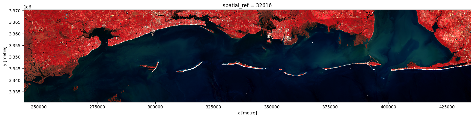
Downloading and preprocessing a single image

Now that the query has returned results, the resulting GeoDataFrame can be used to download and preprocess the imagery using pcx.prepare_data. This function takes all items in a given GeoDataFrame, downloads the imagery, mosaics them (if necessary), resamples and/or reprojects the imagery to match the CRS of the geometry (if necessary), then clips the imagery to the geometry. The result is a single xarray DataArray containing the imagery for the entire geometry, with all bands included.

Looking at the GeoDataFrame of harmonized Sentinel-2 imagery, the first 3 items of 2024 are captured on the same day, so they are suitable for mosaicing. The pcx.prepare_data function handles most of the heavy lifting, but can be supplied with optional arguments to adjust the resampling method (i.e., nearest neighbor, bilinear, etc.), the mosaicing method (i.e., first, last, min, max, mean, median, etc.), the desired resolution, chunking behavior, multiprocessing, and more. The docstring for pcx.prepare_data contains a full list of available arguments and their descriptions.

# selected the first timestep
print(pcx.prepare_data.__doc__)

# The input to prepare_data *must* be a GeoDataFrame with a 'geometry' column
selected_s30_items_gdf = s30_items_gdf.iloc[:3].copy()

s2_image = pcx.prepare_data(
    selected_s30_items_gdf,
    geometry=roi_geom,
    crs=utm_16n_crs,
    bands=['B8A', 'B04', 'B03'],  # NIR, Red, Green
    target_resolution=10.0, # Upsample to 10m resolution (just for demonstration purposes),
    merge_method='mean',  # Use the mean of overlapping pixels
    resampling_method='bilinear',  # Resample using bilinear interpolation
    max_workers=-1,  # Use all available CPU cores for parallel processing
)

aspect = s2_image.shape[2] / s2_image.shape[1]  # Calculate aspect ratio based on the image dimensions
s2_image.plot.imshow(size=4, aspect=aspect, vmin=0, vmax=3000)

    Prepare and merge raster data from Planetary Computer query results.

    This function selects the minimum set of STAC items needed to cover a given geometry,
    reads and mosaics raster tiles, and handles reprojection, resampling, and merging.
    Items are selected using a greedy algorithm to minimize the number of tiles while
    ensuring complete coverage. When a single item fully covers the geometry, no merging
    is performed for efficiency.

    Parameters
    ----------
    items_gdf : geopandas.GeoDataFrame
        GeoDataFrame of STAC items to process.
    geometry : shapely.geometry.base.BaseGeometry
        Area of interest geometry in the target CRS.
    crs : pyproj.CRS, str, or int, default 4326
        Coordinate reference system for the output.
    bands : list of str or int, optional
        List of band names or indices to select; if None, all valid bands are loaded.
    target_resolution : float or int, optional
        Target pixel size for the output raster in units of the CRS. If None, uses the native resolution of the first item.
    all_touched : bool, default False
        Whether to include all pixels touched by the geometry during final clipping.
    merge_method : str, default 'last'
        Method to use when merging overlapping arrays. Options: 'last', 'first', 'min', 'max', 'mean', 'sum', 'median'.
    resampling_method : rasterio.enums.Resampling or str, default 'nearest'
        Resampling method to use for reprojection.
    chunks : str or dict, optional
        Chunking options for dask/xarray.
    enable_time_dim : bool, default False
        If True, add a time dimension to the output. All selected items must have the same datetime value.
    time_col : str, default 'properties.datetime'
        Column name for datetime in items_gdf.
    time_format_str : str, optional
        Format string for parsing datetime values.
    max_workers : int, default 1
        Number of parallel workers to use (-1 uses all available CPUs).
    enable_progress_bar : bool, default False
        Whether to display a progress bar during tile merging.
    **rioxarray_kwargs : dict, optional
        Additional keyword arguments to pass to rioxarray.open_rasterio.

    Returns
    -------
    xarray.DataArray
        The prepared raster data as an xarray DataArray, optionally with a time dimension.

    Raises
    ------
    ValueError
        If enable_time_dim is True but time_col is not found in items_gdf, or if selected items have different datetime values when enable_time_dim is True.

<matplotlib.image.AxesImage at 0x74c4ebb7e480>

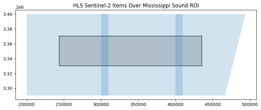
Occasionally, it may be valuable to look at the extent of each item in the collection to see how they overlap with the geometry of interest. As the results of the query are returned as a GeoDataFrame, this can be accomplished using the plot method from GeoPandas.

import matplotlib.pyplot as plt

fig, ax = plt.subplots(figsize=(10, 10))

ms_sound_gdf.plot(ax=ax, color='lightgray', edgecolor='black')
selected_s30_items_gdf.plot(ax=ax, alpha=0.2)

ax.set_title("HLS Sentinel-2 Items Over Mississippi Sound ROI")
plt.show()

An addendum - query_and_prepare

In addition to the pcx.prepare_data function, pcxarray also provides a convenience function called pcx.query_and_prepare. This function combines the querying and preparation steps into a single function call, which can be useful for quickly getting started with a new dataset. The usage is similar to pcx.prepare_data, but it takes the collection ID and datetime range as additional arguments.

s2_image = pcx.query_and_prepare(
    collections=hls_sentinel_collection_id,
    geometry=roi_geom,
    datetime='2024-01-02',
    crs=utm_16n_crs,
    bands=['B8A', 'B04', 'B03'],  # NIR, Red, Green
    target_resolution=10.0,  # Upsample to 10m resolution (just for demonstration purposes),
    merge_method='mean',  # Use the mean of overlapping pixels
    resampling_method='bilinear',  # Resample using bilinear interpolation
    max_workers=-1,  # Use all available CPU cores for parallel processing
)

# Output should be the same as above
aspect = s2_image.shape[2] / s2_image.shape[1]
s2_image.plot.imshow(size=4, aspect=aspect, vmin=0, vmax=3000)

<matplotlib.image.AxesImage at 0x74c541dd6930>

Preparing a time series

For satellite data in particular, preparing a time series of reflectance values is a common task. pcxarray provides a convenient function for this called pcx.prepare_timeseries, which wraps around the pcx.prepare_data function to handle multiple items in a GeoDataFrame and return a single xarray DataArray containing the time series of reflectance values for each band. This function can be used to prepare a time series of data for a given geometry, CRS, and list of bands based on the items provided in a GeoDataFrame.

By default, individual timesteps are processed on a per-date basis, meaning that if multiple items are available for a given date, they will be mosaicked together using the specified mosaicing method (though this functionality can be disabled using ignore_time_component=True if not necessary). Like pcx.prepare_data, pcx.prepare_timeseries can be supplied with optional arguments to adjust the resampling method, mosaicing method, desired resolution, chunking behavior, multiprocessing, and more.

Due to the often large size of time series datasets, it is highly recommended to use the chunks argument to specify how the data should be chunked for processing. Due to how pcxarray works, chunking is best supported along the x and y dimensions of a DataArray, so the best way to handle chunking is to provide a dictionary with the keys x and y and the desired chunk sizes in each dimension. For most cases over relatively small geometries or for relatively coarse data, using chunks={'x': -1, 'y': -1} is sufficient, which will chunk the data into a single chunk along the spatial dimensions. Playing around with the chunk sizes can have a performance impact, so it may be worth experimenting with different chunk sizes to find the best performance for a specific use case. Chunking along the time or band dimensions is supported, but will either trigger a rechunking operation or add an additional rechunking node to the Dask computation graph, which can lead to increased memory usage or slower performance in certain cases (this is highly dataset dependent).

Further, to take advantage of Dask’s parallel processing capabilities, using a Dask local cluster is also recommended. Information on how to install and use the Dask distributed scheduler can be found in the Dask documentation. A minimal example is shown below, which is sufficient for most use cases. Note that the processes=True argument is used to force the scheduler to use processes instead of threads, as using threads can sometimes lead to Dask tasks becoming stuck or failing, potentially due to a lack of thread safety in GDAL (though the exact cause of this is not fully understood).

from distributed import Client
import os

client = Client(n_workers=os.cpu_count(), processes=True)
print(f"Dask client dashboard: {client.dashboard_link}")

Dask client dashboard: http://127.0.0.1:8787/status

2025-07-09 18:53:11,326 - distributed.shuffle._scheduler_plugin - WARNING - Shuffle f9bf80a15f727ed79d29399d4ff2654e initialized by task ('rechunk-merge-rechunk-transfer-6171b91291df20022b0eea6c83d0b5b5', 0, 0, 0, 0, 0, 31) executed on worker tcp://127.0.0.1:40753
2025-07-09 18:57:39,521 - distributed.shuffle._scheduler_plugin - WARNING - Shuffle f9bf80a15f727ed79d29399d4ff2654e deactivated due to stimulus 'task-finished-1752105450.6510918'

s30_da = pcx.prepare_timeseries(
    items_gdf=s30_items_gdf,
    bands=["B03", "B04", "Fmask"],
    geometry=roi_geom,
    crs=utm_16n_crs,
    chunks={"x": -1, "y": -1},  # specify chunk size for dask
    max_workers=-1,  # use all available workers
)
display(s30_da)

l30_da = pcx.prepare_timeseries(
    items_gdf=l30_items_gdf,
    bands=["B03", "B04", "Fmask"],
    geometry=roi_geom,
    crs=utm_16n_crs,
    chunks={"x": -1, "y": -1},
    max_workers=-1,
)
display(l30_da)

Constructing dask computation graph: 100%|██████████| 166/166 [00:09<00:00, 16.80timestep/s]

<xarray.DataArray 'reproject-1e414d34767743ac8b2e4ee6234416f2' (time: 166,
                                                                band: 3,
                                                                y: 1330, x: 6399)> Size: 17GB
dask.array<getitem, shape=(166, 3, 1330, 6399), dtype=float32, chunksize=(1, 1, 1330, 6399), chunktype=numpy.ndarray>
Coordinates:
  * time         (time) datetime64[ns] 1kB 2024-01-02 2024-01-04 ... 2024-12-30
  * band         (band) <U5 60B 'B03' 'B04' 'Fmask'
  * y            (y) float64 11kB 3.37e+06 3.37e+06 ... 3.331e+06 3.331e+06
  * x            (x) float64 51kB 2.435e+05 2.435e+05 ... 4.354e+05 4.354e+05
    spatial_ref  int32 4B 32616
Attributes: (12/42)
    ACCODE:                                            LaSRC
    add_offset:                                        0.0
    arop_ave_xshift(meters):                           0
    arop_ave_yshift(meters):                           0
    arop_ncp:                                          0
    arop_rmse(meters):                                 0
    ...                                                ...
    SPATIAL_RESOLUTION:                                30
    TILE_ID:                                           S2A_OPER_MSI_L1C_TL_2A...
    ULX:                                               399960
    ULY:                                               3400020
    AREA_OR_POINT:                                     Area
    _FillValue:                                        nan

xarray.DataArray

'reproject-1e414d34767743ac8b2e4ee6234416f2'

• time: 166
• band: 3
• y: 1330
• x: 6399

• dask.array<chunksize=(1, 1, 1330, 6399), meta=np.ndarray>

  Array Chunk Bytes 15.79 GiB 32.47 MiB Shape (166, 3, 1330, 6399) (1, 1, 1330, 6399) Dask graph 498 chunks in 4720 graph layers Data type float32 numpy.ndarray

• Coordinates: (5)
  • time
    (time)
    datetime64[ns]
    2024-01-02 ... 2024-12-30

    array(['2024-01-02T00:00:00.000000000', '2024-01-04T00:00:00.000000000',
           '2024-01-07T00:00:00.000000000', '2024-01-09T00:00:00.000000000',
           '2024-01-10T00:00:00.000000000', '2024-01-12T00:00:00.000000000',
           '2024-01-14T00:00:00.000000000', '2024-01-15T00:00:00.000000000',
           '2024-01-17T00:00:00.000000000', '2024-01-19T00:00:00.000000000',
           '2024-01-20T00:00:00.000000000', '2024-01-22T00:00:00.000000000',
           '2024-01-24T00:00:00.000000000', '2024-01-29T00:00:00.000000000',
           '2024-01-30T00:00:00.000000000', '2024-02-01T00:00:00.000000000',
           '2024-02-04T00:00:00.000000000', '2024-02-06T00:00:00.000000000',
           '2024-02-08T00:00:00.000000000', '2024-02-09T00:00:00.000000000',
           '2024-02-13T00:00:00.000000000', '2024-02-14T00:00:00.000000000',
           '2024-02-19T00:00:00.000000000', '2024-02-21T00:00:00.000000000',
           '2024-02-23T00:00:00.000000000', '2024-02-24T00:00:00.000000000',
           '2024-02-26T00:00:00.000000000', '2024-02-28T00:00:00.000000000',
           '2024-03-02T00:00:00.000000000', '2024-03-04T00:00:00.000000000',
           '2024-03-07T00:00:00.000000000', '2024-03-10T00:00:00.000000000',
           '2024-03-12T00:00:00.000000000', '2024-03-14T00:00:00.000000000',
           '2024-03-15T00:00:00.000000000', '2024-03-19T00:00:00.000000000',
           '2024-03-20T00:00:00.000000000', '2024-03-22T00:00:00.000000000',
           '2024-03-24T00:00:00.000000000', '2024-03-27T00:00:00.000000000',
           '2024-03-29T00:00:00.000000000', '2024-03-30T00:00:00.000000000',
           '2024-04-03T00:00:00.000000000', '2024-04-06T00:00:00.000000000',
           '2024-04-08T00:00:00.000000000', '2024-04-11T00:00:00.000000000',
           '2024-04-13T00:00:00.000000000', '2024-04-14T00:00:00.000000000',
           '2024-04-16T00:00:00.000000000', '2024-04-18T00:00:00.000000000',
           '2024-04-21T00:00:00.000000000', '2024-04-23T00:00:00.000000000',
           '2024-04-24T00:00:00.000000000', '2024-04-26T00:00:00.000000000',
           '2024-04-28T00:00:00.000000000', '2024-05-01T00:00:00.000000000',
           '2024-05-03T00:00:00.000000000', '2024-05-04T00:00:00.000000000',
           '2024-05-06T00:00:00.000000000', '2024-05-08T00:00:00.000000000',
           '2024-05-09T00:00:00.000000000', '2024-05-11T00:00:00.000000000',
           '2024-05-16T00:00:00.000000000', '2024-05-19T00:00:00.000000000',
           '2024-05-21T00:00:00.000000000', '2024-05-23T00:00:00.000000000',
           '2024-05-24T00:00:00.000000000', '2024-05-26T00:00:00.000000000',
           '2024-05-28T00:00:00.000000000', '2024-05-31T00:00:00.000000000',
           '2024-06-02T00:00:00.000000000', '2024-06-05T00:00:00.000000000',
           '2024-06-07T00:00:00.000000000', '2024-06-08T00:00:00.000000000',
           '2024-06-10T00:00:00.000000000', '2024-06-12T00:00:00.000000000',
           '2024-06-30T00:00:00.000000000', '2024-07-02T00:00:00.000000000',
           '2024-07-03T00:00:00.000000000', '2024-07-05T00:00:00.000000000',
           '2024-07-07T00:00:00.000000000', '2024-07-08T00:00:00.000000000',
           '2024-07-10T00:00:00.000000000', '2024-07-12T00:00:00.000000000',
           '2024-07-13T00:00:00.000000000', '2024-07-15T00:00:00.000000000',
           '2024-07-17T00:00:00.000000000', '2024-07-18T00:00:00.000000000',
           '2024-07-20T00:00:00.000000000', '2024-07-22T00:00:00.000000000',
           '2024-07-25T00:00:00.000000000', '2024-07-27T00:00:00.000000000',
           '2024-07-28T00:00:00.000000000', '2024-07-30T00:00:00.000000000',
           '2024-08-01T00:00:00.000000000', '2024-08-02T00:00:00.000000000',
           '2024-08-04T00:00:00.000000000', '2024-08-06T00:00:00.000000000',
           '2024-08-07T00:00:00.000000000', '2024-08-09T00:00:00.000000000',
           '2024-08-11T00:00:00.000000000', '2024-08-12T00:00:00.000000000',
           '2024-08-14T00:00:00.000000000', '2024-08-16T00:00:00.000000000',
           '2024-08-17T00:00:00.000000000', '2024-08-19T00:00:00.000000000',
           '2024-08-21T00:00:00.000000000', '2024-08-22T00:00:00.000000000',
           '2024-08-24T00:00:00.000000000', '2024-08-26T00:00:00.000000000',
           '2024-08-27T00:00:00.000000000', '2024-08-29T00:00:00.000000000',
           '2024-09-03T00:00:00.000000000', '2024-09-08T00:00:00.000000000',
           '2024-09-13T00:00:00.000000000', '2024-09-15T00:00:00.000000000',
           '2024-09-18T00:00:00.000000000', '2024-09-20T00:00:00.000000000',
           '2024-09-23T00:00:00.000000000', '2024-09-25T00:00:00.000000000',
           '2024-09-26T00:00:00.000000000', '2024-09-28T00:00:00.000000000',
           '2024-09-30T00:00:00.000000000', '2024-10-01T00:00:00.000000000',
           '2024-10-03T00:00:00.000000000', '2024-10-05T00:00:00.000000000',
           '2024-10-06T00:00:00.000000000', '2024-10-08T00:00:00.000000000',
           '2024-10-10T00:00:00.000000000', '2024-10-11T00:00:00.000000000',
           '2024-10-13T00:00:00.000000000', '2024-10-15T00:00:00.000000000',
           '2024-10-18T00:00:00.000000000', '2024-10-20T00:00:00.000000000',
           '2024-10-21T00:00:00.000000000', '2024-10-23T00:00:00.000000000',
           '2024-10-25T00:00:00.000000000', '2024-10-28T00:00:00.000000000',
           '2024-10-30T00:00:00.000000000', '2024-10-31T00:00:00.000000000',
           '2024-11-02T00:00:00.000000000', '2024-11-04T00:00:00.000000000',
           '2024-11-05T00:00:00.000000000', '2024-11-07T00:00:00.000000000',
           '2024-11-12T00:00:00.000000000', '2024-11-14T00:00:00.000000000',
           '2024-11-15T00:00:00.000000000', '2024-11-17T00:00:00.000000000',
           '2024-11-22T00:00:00.000000000', '2024-11-24T00:00:00.000000000',
           '2024-11-27T00:00:00.000000000', '2024-11-29T00:00:00.000000000',
           '2024-11-30T00:00:00.000000000', '2024-12-04T00:00:00.000000000',
           '2024-12-07T00:00:00.000000000', '2024-12-10T00:00:00.000000000',
           '2024-12-12T00:00:00.000000000', '2024-12-14T00:00:00.000000000',
           '2024-12-15T00:00:00.000000000', '2024-12-17T00:00:00.000000000',
           '2024-12-20T00:00:00.000000000', '2024-12-22T00:00:00.000000000',
           '2024-12-24T00:00:00.000000000', '2024-12-27T00:00:00.000000000',
           '2024-12-29T00:00:00.000000000', '2024-12-30T00:00:00.000000000'],
          dtype='datetime64[ns]')

  • band
    (band)
    <U5
    'B03' 'B04' 'Fmask'

    array(['B03', 'B04', 'Fmask'], dtype='<U5')

  • y
    (y)
    float64
    3.37e+06 3.37e+06 ... 3.331e+06

    units :

    metre

    resolution :

    -30.0

    crs :

    EPSG:32616

    array([3370395., 3370365., 3370335., ..., 3330585., 3330555., 3330525.],
          shape=(1330,))

  • x
    (x)
    float64
    2.435e+05 2.435e+05 ... 4.354e+05

    units :

    metre

    resolution :

    30.0

    crs :

    EPSG:32616

    array([243495., 243525., 243555., ..., 435375., 435405., 435435.],
          shape=(6399,))

  • spatial_ref
    ()
    int32
    32616

    spatial_ref :

    PROJCRS["WGS 84 / UTM zone 16N",BASEGEOGCRS["WGS 84",ENSEMBLE["World Geodetic System 1984 ensemble",MEMBER["World Geodetic System 1984 (Transit)"],MEMBER["World Geodetic System 1984 (G730)"],MEMBER["World Geodetic System 1984 (G873)"],MEMBER["World Geodetic System 1984 (G1150)"],MEMBER["World Geodetic System 1984 (G1674)"],MEMBER["World Geodetic System 1984 (G1762)"],MEMBER["World Geodetic System 1984 (G2139)"],MEMBER["World Geodetic System 1984 (G2296)"],ELLIPSOID["WGS 84",6378137,298.257223563,LENGTHUNIT["metre",1]],ENSEMBLEACCURACY[2.0]],PRIMEM["Greenwich",0,ANGLEUNIT["degree",0.0174532925199433]],ID["EPSG",4326]],CONVERSION["UTM zone 16N",METHOD["Transverse Mercator",ID["EPSG",9807]],PARAMETER["Latitude of natural origin",0,ANGLEUNIT["degree",0.0174532925199433],ID["EPSG",8801]],PARAMETER["Longitude of natural origin",-87,ANGLEUNIT["degree",0.0174532925199433],ID["EPSG",8802]],PARAMETER["Scale factor at natural origin",0.9996,SCALEUNIT["unity",1],ID["EPSG",8805]],PARAMETER["False easting",500000,LENGTHUNIT["metre",1],ID["EPSG",8806]],PARAMETER["False northing",0,LENGTHUNIT["metre",1],ID["EPSG",8807]]],CS[Cartesian,2],AXIS["(E)",east,ORDER[1],LENGTHUNIT["metre",1]],AXIS["(N)",north,ORDER[2],LENGTHUNIT["metre",1]],USAGE[SCOPE["Navigation and medium accuracy spatial referencing."],AREA["Between 90°W and 84°W, northern hemisphere between equator and 84°N, onshore and offshore. Belize. Canada - Manitoba; Nunavut; Ontario. Costa Rica. Cuba. Ecuador - Galapagos. El Salvador. Guatemala. Honduras. Mexico. Nicaragua. United States (USA)."],BBOX[0,-90,84,-84]],ID["EPSG",32616]]

    crs_wkt :

    PROJCRS["WGS 84 / UTM zone 16N",BASEGEOGCRS["WGS 84",ENSEMBLE["World Geodetic System 1984 ensemble",MEMBER["World Geodetic System 1984 (Transit)"],MEMBER["World Geodetic System 1984 (G730)"],MEMBER["World Geodetic System 1984 (G873)"],MEMBER["World Geodetic System 1984 (G1150)"],MEMBER["World Geodetic System 1984 (G1674)"],MEMBER["World Geodetic System 1984 (G1762)"],MEMBER["World Geodetic System 1984 (G2139)"],MEMBER["World Geodetic System 1984 (G2296)"],ELLIPSOID["WGS 84",6378137,298.257223563,LENGTHUNIT["metre",1]],ENSEMBLEACCURACY[2.0]],PRIMEM["Greenwich",0,ANGLEUNIT["degree",0.0174532925199433]],ID["EPSG",4326]],CONVERSION["UTM zone 16N",METHOD["Transverse Mercator",ID["EPSG",9807]],PARAMETER["Latitude of natural origin",0,ANGLEUNIT["degree",0.0174532925199433],ID["EPSG",8801]],PARAMETER["Longitude of natural origin",-87,ANGLEUNIT["degree",0.0174532925199433],ID["EPSG",8802]],PARAMETER["Scale factor at natural origin",0.9996,SCALEUNIT["unity",1],ID["EPSG",8805]],PARAMETER["False easting",500000,LENGTHUNIT["metre",1],ID["EPSG",8806]],PARAMETER["False northing",0,LENGTHUNIT["metre",1],ID["EPSG",8807]]],CS[Cartesian,2],AXIS["(E)",east,ORDER[1],LENGTHUNIT["metre",1]],AXIS["(N)",north,ORDER[2],LENGTHUNIT["metre",1]],USAGE[SCOPE["Navigation and medium accuracy spatial referencing."],AREA["Between 90°W and 84°W, northern hemisphere between equator and 84°N, onshore and offshore. Belize. Canada - Manitoba; Nunavut; Ontario. Costa Rica. Cuba. Ecuador - Galapagos. El Salvador. Guatemala. Honduras. Mexico. Nicaragua. United States (USA)."],BBOX[0,-90,84,-84]],ID["EPSG",32616]]

    semi_major_axis :

    6378137.0

    semi_minor_axis :

    6356752.314245179

    inverse_flattening :

    298.257223563

    reference_ellipsoid_name :

    WGS 84

    longitude_of_prime_meridian :

    0.0

    prime_meridian_name :

    Greenwich

    geographic_crs_name :

    WGS 84

    horizontal_datum_name :

    World Geodetic System 1984 ensemble

    projected_crs_name :

    WGS 84 / UTM zone 16N

    grid_mapping_name :

    transverse_mercator

    latitude_of_projection_origin :

    0.0

    longitude_of_central_meridian :

    -87.0

    false_easting :

    500000.0

    false_northing :

    0.0

    scale_factor_at_central_meridian :

    0.9996

    GeoTransform :

    243480 30 0 3370410 0 -30

    array(32616, dtype=int32)

• Indexes: (4)
  • time
    PandasIndex

    PandasIndex(DatetimeIndex(['2024-01-02', '2024-01-04', '2024-01-07', '2024-01-09',
                   '2024-01-10', '2024-01-12', '2024-01-14', '2024-01-15',
                   '2024-01-17', '2024-01-19',
                   ...
                   '2024-12-12', '2024-12-14', '2024-12-15', '2024-12-17',
                   '2024-12-20', '2024-12-22', '2024-12-24', '2024-12-27',
                   '2024-12-29', '2024-12-30'],
                  dtype='datetime64[ns]', name='time', length=166, freq=None))

  • band
    PandasIndex

    PandasIndex(Index(['B03', 'B04', 'Fmask'], dtype='object', name='band'))

  • y
    PandasIndex

    PandasIndex(Index([3370395.0, 3370365.0, 3370335.0, 3370305.0, 3370275.0, 3370245.0,
           3370215.0, 3370185.0, 3370155.0, 3370125.0,
           ...
           3330795.0, 3330765.0, 3330735.0, 3330705.0, 3330675.0, 3330645.0,
           3330615.0, 3330585.0, 3330555.0, 3330525.0],
          dtype='float64', name='y', length=1330))

  • x
    PandasIndex

    PandasIndex(Index([243495.0, 243525.0, 243555.0, 243585.0, 243615.0, 243645.0, 243675.0,
           243705.0, 243735.0, 243765.0,
           ...
           435165.0, 435195.0, 435225.0, 435255.0, 435285.0, 435315.0, 435345.0,
           435375.0, 435405.0, 435435.0],
          dtype='float64', name='x', length=6399))

• Attributes: (42)

  ACCODE :

  LaSRC

  add_offset :

  0.0

  arop_ave_xshift(meters) :

  0

  arop_ave_yshift(meters) :

  0

  arop_ncp :

  0

  arop_rmse(meters) :

  0

  arop_s2_refimg :

  NONE

  cloud_coverage :

  7

  DATASTRIP_ID :

  S2A_OPER_MSI_L1C_DS_2APS_20240102T183340_S20240102T164358_N05.10

  HLS_PROCESSING_TIME :

  2024-01-08T22:29:27Z

  HORIZONTAL_CS_CODE :

  EPSG:32616

  HORIZONTAL_CS_NAME :

  WGS84 / UTM zone 16N

  L1C_IMAGE_QUALITY :

  NONE

  L1_PROCESSING_TIME :

  2024-01-02T19:49:37.462667Z

  long_name :

  Green

  MEAN_SUN_AZIMUTH_ANGLE :

  160.612734083722

  MEAN_SUN_ZENITH_ANGLE :

  55.7071929243025

  MEAN_VIEW_AZIMUTH_ANGLE :

  286.178866435583

  MEAN_VIEW_ZENITH_ANGLE :

  8.75212644272923

  MSI band 01 bandpass adjustment slope and offset :

  0.995900, -0.000200

  MSI band 02 bandpass adjustment slope and offset :

  0.977800, -0.004000

  MSI band 03 bandpass adjustment slope and offset :

  1.005300, -0.000900

  MSI band 04 bandpass adjustment slope and offset :

  0.976500, 0.000900

  MSI band 11 bandpass adjustment slope and offset :

  0.998700, -0.001100

  MSI band 12 bandpass adjustment slope and offset :

  1.003000, -0.001200

  MSI band 8a bandpass adjustment slope and offset :

  0.998300, -0.000100

  NBAR_SOLAR_ZENITH :

  56.8646255518341

  NCOLS :

  3660

  NROWS :

  3660

  OVR_RESAMPLING_ALG :

  NEAREST

  PROCESSING_BASELINE :

  5.1

  PRODUCT_URI :

  S2A_MSIL1C_20240102T163701_N0510_R083_T16RDU_20240102T183340.SAFE

  scale_factor :

  0.0001

  SENSING_TIME :

  2024-01-02T16:45:03.872012Z

  SPACECRAFT_NAME :

  Sentinel-2A

  spatial_coverage :

  73

  SPATIAL_RESOLUTION :

  30

  TILE_ID :

  S2A_OPER_MSI_L1C_TL_2APS_20240102T183340_A044553_T16RDU_N05.10

  ULX :

  399960

  ULY :

  3400020

  AREA_OR_POINT :

  Area

  _FillValue :

  nan

Constructing dask computation graph: 100%|██████████| 113/113 [00:03<00:00, 28.71timestep/s]

<xarray.DataArray 'reproject-b55a2cb0d7874ebb8e0de5a299422ff3' (time: 113,
                                                                band: 3,
                                                                y: 1330, x: 6399)> Size: 12GB
dask.array<getitem, shape=(113, 3, 1330, 6399), dtype=float32, chunksize=(1, 1, 1330, 6399), chunktype=numpy.ndarray>
Coordinates:
  * time         (time) datetime64[ns] 904B 2024-01-01 2024-01-07 ... 2024-12-25
  * band         (band) <U5 60B 'B03' 'B04' 'Fmask'
  * y            (y) float64 11kB 3.37e+06 3.37e+06 ... 3.331e+06 3.331e+06
  * x            (x) float64 51kB 2.435e+05 2.435e+05 ... 4.354e+05 4.354e+05
    spatial_ref  int32 4B 32616
Attributes: (12/36)
    ACCODE:                    Lasrc
    add_offset:                0.0
    arop_ave_xshift(meters):   0
    arop_ave_yshift(meters):   0
    arop_ncp:                  0
    arop_rmse(meters):         0
    ...                        ...
    TIRS_SSM_POSITION_STATUS:  ESTIMATED
    ULX:                       300000
    ULY:                       3400020
    USGS_SOFTWARE:             LPGS_16.3.1
    AREA_OR_POINT:             Area
    _FillValue:                nan

xarray.DataArray

'reproject-b55a2cb0d7874ebb8e0de5a299422ff3'

• time: 113
• band: 3
• y: 1330
• x: 6399

• dask.array<chunksize=(1, 1, 1330, 6399), meta=np.ndarray>

  Array Chunk Bytes 10.75 GiB 32.47 MiB Shape (113, 3, 1330, 6399) (1, 1, 1330, 6399) Dask graph 339 chunks in 3658 graph layers Data type float32 numpy.ndarray

• Coordinates: (5)
  • time
    (time)
    datetime64[ns]
    2024-01-01 ... 2024-12-25

    array(['2024-01-01T00:00:00.000000000', '2024-01-07T00:00:00.000000000',
           '2024-01-15T00:00:00.000000000', '2024-01-16T00:00:00.000000000',
           '2024-01-17T00:00:00.000000000', '2024-01-23T00:00:00.000000000',
           '2024-01-24T00:00:00.000000000', '2024-01-31T00:00:00.000000000',
           '2024-02-01T00:00:00.000000000', '2024-02-02T00:00:00.000000000',
           '2024-02-08T00:00:00.000000000', '2024-02-09T00:00:00.000000000',
           '2024-02-18T00:00:00.000000000', '2024-02-24T00:00:00.000000000',
           '2024-02-25T00:00:00.000000000', '2024-02-26T00:00:00.000000000',
           '2024-03-03T00:00:00.000000000', '2024-03-11T00:00:00.000000000',
           '2024-03-12T00:00:00.000000000', '2024-03-13T00:00:00.000000000',
           '2024-03-19T00:00:00.000000000', '2024-03-20T00:00:00.000000000',
           '2024-03-21T00:00:00.000000000', '2024-03-27T00:00:00.000000000',
           '2024-03-28T00:00:00.000000000', '2024-03-29T00:00:00.000000000',
           '2024-04-04T00:00:00.000000000', '2024-04-05T00:00:00.000000000',
           '2024-04-06T00:00:00.000000000', '2024-04-12T00:00:00.000000000',
           '2024-04-13T00:00:00.000000000', '2024-04-14T00:00:00.000000000',
           '2024-04-20T00:00:00.000000000', '2024-04-22T00:00:00.000000000',
           '2024-04-28T00:00:00.000000000', '2024-04-29T00:00:00.000000000',
           '2024-04-30T00:00:00.000000000', '2024-05-06T00:00:00.000000000',
           '2024-05-07T00:00:00.000000000', '2024-05-08T00:00:00.000000000',
           '2024-05-14T00:00:00.000000000', '2024-05-15T00:00:00.000000000',
           '2024-05-16T00:00:00.000000000', '2024-05-22T00:00:00.000000000',
           '2024-05-23T00:00:00.000000000', '2024-05-24T00:00:00.000000000',
           '2024-05-30T00:00:00.000000000', '2024-05-31T00:00:00.000000000',
           '2024-06-01T00:00:00.000000000', '2024-06-07T00:00:00.000000000',
           '2024-06-08T00:00:00.000000000', '2024-06-09T00:00:00.000000000',
           '2024-07-01T00:00:00.000000000', '2024-07-02T00:00:00.000000000',
           '2024-07-03T00:00:00.000000000', '2024-07-09T00:00:00.000000000',
           '2024-07-10T00:00:00.000000000', '2024-07-11T00:00:00.000000000',
           '2024-07-17T00:00:00.000000000', '2024-07-18T00:00:00.000000000',
           '2024-07-25T00:00:00.000000000', '2024-07-26T00:00:00.000000000',
           '2024-07-27T00:00:00.000000000', '2024-08-02T00:00:00.000000000',
           '2024-08-03T00:00:00.000000000', '2024-08-04T00:00:00.000000000',
           '2024-08-10T00:00:00.000000000', '2024-08-11T00:00:00.000000000',
           '2024-08-12T00:00:00.000000000', '2024-08-18T00:00:00.000000000',
           '2024-08-19T00:00:00.000000000', '2024-08-20T00:00:00.000000000',
           '2024-08-26T00:00:00.000000000', '2024-08-27T00:00:00.000000000',
           '2024-08-28T00:00:00.000000000', '2024-09-03T00:00:00.000000000',
           '2024-09-04T00:00:00.000000000', '2024-09-12T00:00:00.000000000',
           '2024-09-13T00:00:00.000000000', '2024-09-19T00:00:00.000000000',
           '2024-09-20T00:00:00.000000000', '2024-09-21T00:00:00.000000000',
           '2024-09-27T00:00:00.000000000', '2024-09-28T00:00:00.000000000',
           '2024-09-29T00:00:00.000000000', '2024-10-05T00:00:00.000000000',
           '2024-10-06T00:00:00.000000000', '2024-10-07T00:00:00.000000000',
           '2024-10-13T00:00:00.000000000', '2024-10-14T00:00:00.000000000',
           '2024-10-21T00:00:00.000000000', '2024-10-22T00:00:00.000000000',
           '2024-10-23T00:00:00.000000000', '2024-10-29T00:00:00.000000000',
           '2024-10-30T00:00:00.000000000', '2024-10-31T00:00:00.000000000',
           '2024-11-06T00:00:00.000000000', '2024-11-14T00:00:00.000000000',
           '2024-11-15T00:00:00.000000000', '2024-11-16T00:00:00.000000000',
           '2024-11-22T00:00:00.000000000', '2024-11-23T00:00:00.000000000',
           '2024-11-24T00:00:00.000000000', '2024-11-30T00:00:00.000000000',
           '2024-12-01T00:00:00.000000000', '2024-12-02T00:00:00.000000000',
           '2024-12-08T00:00:00.000000000', '2024-12-10T00:00:00.000000000',
           '2024-12-16T00:00:00.000000000', '2024-12-17T00:00:00.000000000',
           '2024-12-18T00:00:00.000000000', '2024-12-24T00:00:00.000000000',
           '2024-12-25T00:00:00.000000000'], dtype='datetime64[ns]')

  • band
    (band)
    <U5
    'B03' 'B04' 'Fmask'

    array(['B03', 'B04', 'Fmask'], dtype='<U5')

  • y
    (y)
    float64
    3.37e+06 3.37e+06 ... 3.331e+06

    units :

    metre

    resolution :

    -30.0

    crs :

    EPSG:32616

    array([3370395., 3370365., 3370335., ..., 3330585., 3330555., 3330525.],
          shape=(1330,))

  • x
    (x)
    float64
    2.435e+05 2.435e+05 ... 4.354e+05

    units :

    metre

    resolution :

    30.0

    crs :

    EPSG:32616

    array([243495., 243525., 243555., ..., 435375., 435405., 435435.],
          shape=(6399,))

  • spatial_ref
    ()
    int32
    32616

    spatial_ref :

    PROJCRS["WGS 84 / UTM zone 16N",BASEGEOGCRS["WGS 84",ENSEMBLE["World Geodetic System 1984 ensemble",MEMBER["World Geodetic System 1984 (Transit)"],MEMBER["World Geodetic System 1984 (G730)"],MEMBER["World Geodetic System 1984 (G873)"],MEMBER["World Geodetic System 1984 (G1150)"],MEMBER["World Geodetic System 1984 (G1674)"],MEMBER["World Geodetic System 1984 (G1762)"],MEMBER["World Geodetic System 1984 (G2139)"],MEMBER["World Geodetic System 1984 (G2296)"],ELLIPSOID["WGS 84",6378137,298.257223563,LENGTHUNIT["metre",1]],ENSEMBLEACCURACY[2.0]],PRIMEM["Greenwich",0,ANGLEUNIT["degree",0.0174532925199433]],ID["EPSG",4326]],CONVERSION["UTM zone 16N",METHOD["Transverse Mercator",ID["EPSG",9807]],PARAMETER["Latitude of natural origin",0,ANGLEUNIT["degree",0.0174532925199433],ID["EPSG",8801]],PARAMETER["Longitude of natural origin",-87,ANGLEUNIT["degree",0.0174532925199433],ID["EPSG",8802]],PARAMETER["Scale factor at natural origin",0.9996,SCALEUNIT["unity",1],ID["EPSG",8805]],PARAMETER["False easting",500000,LENGTHUNIT["metre",1],ID["EPSG",8806]],PARAMETER["False northing",0,LENGTHUNIT["metre",1],ID["EPSG",8807]]],CS[Cartesian,2],AXIS["(E)",east,ORDER[1],LENGTHUNIT["metre",1]],AXIS["(N)",north,ORDER[2],LENGTHUNIT["metre",1]],USAGE[SCOPE["Navigation and medium accuracy spatial referencing."],AREA["Between 90°W and 84°W, northern hemisphere between equator and 84°N, onshore and offshore. Belize. Canada - Manitoba; Nunavut; Ontario. Costa Rica. Cuba. Ecuador - Galapagos. El Salvador. Guatemala. Honduras. Mexico. Nicaragua. United States (USA)."],BBOX[0,-90,84,-84]],ID["EPSG",32616]]

    crs_wkt :

    PROJCRS["WGS 84 / UTM zone 16N",BASEGEOGCRS["WGS 84",ENSEMBLE["World Geodetic System 1984 ensemble",MEMBER["World Geodetic System 1984 (Transit)"],MEMBER["World Geodetic System 1984 (G730)"],MEMBER["World Geodetic System 1984 (G873)"],MEMBER["World Geodetic System 1984 (G1150)"],MEMBER["World Geodetic System 1984 (G1674)"],MEMBER["World Geodetic System 1984 (G1762)"],MEMBER["World Geodetic System 1984 (G2139)"],MEMBER["World Geodetic System 1984 (G2296)"],ELLIPSOID["WGS 84",6378137,298.257223563,LENGTHUNIT["metre",1]],ENSEMBLEACCURACY[2.0]],PRIMEM["Greenwich",0,ANGLEUNIT["degree",0.0174532925199433]],ID["EPSG",4326]],CONVERSION["UTM zone 16N",METHOD["Transverse Mercator",ID["EPSG",9807]],PARAMETER["Latitude of natural origin",0,ANGLEUNIT["degree",0.0174532925199433],ID["EPSG",8801]],PARAMETER["Longitude of natural origin",-87,ANGLEUNIT["degree",0.0174532925199433],ID["EPSG",8802]],PARAMETER["Scale factor at natural origin",0.9996,SCALEUNIT["unity",1],ID["EPSG",8805]],PARAMETER["False easting",500000,LENGTHUNIT["metre",1],ID["EPSG",8806]],PARAMETER["False northing",0,LENGTHUNIT["metre",1],ID["EPSG",8807]]],CS[Cartesian,2],AXIS["(E)",east,ORDER[1],LENGTHUNIT["metre",1]],AXIS["(N)",north,ORDER[2],LENGTHUNIT["metre",1]],USAGE[SCOPE["Navigation and medium accuracy spatial referencing."],AREA["Between 90°W and 84°W, northern hemisphere between equator and 84°N, onshore and offshore. Belize. Canada - Manitoba; Nunavut; Ontario. Costa Rica. Cuba. Ecuador - Galapagos. El Salvador. Guatemala. Honduras. Mexico. Nicaragua. United States (USA)."],BBOX[0,-90,84,-84]],ID["EPSG",32616]]

    semi_major_axis :

    6378137.0

    semi_minor_axis :

    6356752.314245179

    inverse_flattening :

    298.257223563

    reference_ellipsoid_name :

    WGS 84

    longitude_of_prime_meridian :

    0.0

    prime_meridian_name :

    Greenwich

    geographic_crs_name :

    WGS 84

    horizontal_datum_name :

    World Geodetic System 1984 ensemble

    projected_crs_name :

    WGS 84 / UTM zone 16N

    grid_mapping_name :

    transverse_mercator

    latitude_of_projection_origin :

    0.0

    longitude_of_central_meridian :

    -87.0

    false_easting :

    500000.0

    false_northing :

    0.0

    scale_factor_at_central_meridian :

    0.9996

    GeoTransform :

    243480 30 0 3370410 0 -30

    array(32616, dtype=int32)

• Indexes: (4)
  • time
    PandasIndex

    PandasIndex(DatetimeIndex(['2024-01-01', '2024-01-07', '2024-01-15', '2024-01-16',
                   '2024-01-17', '2024-01-23', '2024-01-24', '2024-01-31',
                   '2024-02-01', '2024-02-02',
                   ...
                   '2024-11-30', '2024-12-01', '2024-12-02', '2024-12-08',
                   '2024-12-10', '2024-12-16', '2024-12-17', '2024-12-18',
                   '2024-12-24', '2024-12-25'],
                  dtype='datetime64[ns]', name='time', length=113, freq=None))

  • band
    PandasIndex

    PandasIndex(Index(['B03', 'B04', 'Fmask'], dtype='object', name='band'))

  • y
    PandasIndex

    PandasIndex(Index([3370395.0, 3370365.0, 3370335.0, 3370305.0, 3370275.0, 3370245.0,
           3370215.0, 3370185.0, 3370155.0, 3370125.0,
           ...
           3330795.0, 3330765.0, 3330735.0, 3330705.0, 3330675.0, 3330645.0,
           3330615.0, 3330585.0, 3330555.0, 3330525.0],
          dtype='float64', name='y', length=1330))

  • x
    PandasIndex

    PandasIndex(Index([243495.0, 243525.0, 243555.0, 243585.0, 243615.0, 243645.0, 243675.0,
           243705.0, 243735.0, 243765.0,
           ...
           435165.0, 435195.0, 435225.0, 435255.0, 435285.0, 435315.0, 435345.0,
           435375.0, 435405.0, 435435.0],
          dtype='float64', name='x', length=6399))

• Attributes: (36)

  ACCODE :

  Lasrc

  add_offset :

  0.0

  arop_ave_xshift(meters) :

  0

  arop_ave_yshift(meters) :

  0

  arop_ncp :

  0

  arop_rmse(meters) :

  0

  arop_s2_refimg :

  NONE

  cloud_coverage :

  1

  HLS_PROCESSING_TIME :

  2024-01-05T00:15:20Z

  HORIZONTAL_CS_NAME :

  UTM, WGS84, UTM ZONE 16

  L1_PROCESSING_TIME :

  2024-01-01T20:01:01Z

  LANDSAT_PRODUCT_ID :

  LC08_L1TP_020039_20240101_20240101_02_RT

  LANDSAT_SCENE_ID :

  LC80200392024001LGN00

  long_name :

  Green

  MEAN_SUN_AZIMUTH_ANGLE :

  153.87987259118

  MEAN_SUN_ZENITH_ANGLE :

  57.7933216520912

  MEAN_VIEW_AZIMUTH_ANGLE :

  102.126991174513

  MEAN_VIEW_ZENITH_ANGLE :

  7.64848856628561

  NBAR_SOLAR_ZENITH :

  56.8981213430387

  NCOLS :

  3660

  NROWS :

  3660

  OVR_RESAMPLING_ALG :

  NEAREST

  PROCESSING_LEVEL :

  L1TP

  scale_factor :

  0.0001

  SENSING_TIME :

  2024-01-01T16:19:51.7008680Z

  SENSOR :

  OLI_TIRS

  SENTINEL2_TILEID :

  16RCU

  spatial_coverage :

  10

  SPATIAL_RESOLUTION :

  30

  TIRS_SSM_MODEL :

  PRELIMINARY

  TIRS_SSM_POSITION_STATUS :

  ESTIMATED

  ULX :

  300000

  ULY :

  3400020

  USGS_SOFTWARE :

  LPGS_16.3.1

  AREA_OR_POINT :

  Area

  _FillValue :

  nan

Dask lazy execution model

Both of the operations above should run relatively quickly, as they are only preparing the Dask computation graphs which involves reading a small amount of metadata from the rasters and creating the necessary Dask arrays, but not actually downloading or processing any data yet. The actual data loading and processing will occur when the Dask computation graph is executed, which can be done at a later time (e.g., by using the compute() method on the resulting DataArray instance).

Full compatibility with Dask’s lazy execution model is a key priority for pcxarray and is one of the main reasons it was created. Unlike most other geospatial libraries that rely on GDAL for data access (and thus breaks Dask’s lazy execution model), pcxarray utilizes odc-geo to handle reprojection and mosaicing of rasters instead, ensuring that the Dask computation graph is not evaluated until it is explicitly requested. This approach allows a user to define a complex processing pipeline where a large dataset undergoes multiple transformations, but does not necessarily require the data to be loaded into memory all at once, rather, it will be loaded in chunks as needed when the computation is executed and discarded once the raw data is no longer needed to produce the final result. For more information on Dask, see the Dask documentation.

Now that both time series DataArrays have been prepared, they can be concatenated together to create a single DataArray containing both the harmonized Sentinel-2 and Landsat time series. While not strictly necessary here, it is good practice to rename the band values to ensure they are consistent with each other before concatenating the arrays. For example, the Sentinel-2 band name for the NIR Narrow band is “B8A”, while Landsat uses “B05” to refer to the same spectral band. To ensure consistency and make things easier, renaming the bands to a common, more descriptive name is recommended.

import xarray as xr

s30_bands_mapping = {
    'B03': 'green',
    'B04': 'red',
    'Fmask': 'fmask'
}
l30_bands_mapping = {
    'B03': 'green',
    'B04': 'red',
    'Fmask': 'fmask'
}

# rename the bands in the data arrays
s30_da = s30_da.assign_coords(band=[s30_bands_mapping[b] for b in s30_da.band.values])
l30_da = l30_da.assign_coords(band=[l30_bands_mapping[b] for b in l30_da.band.values])

da = xr.concat([s30_da, l30_da], dim='time')
da = da.sortby('time')  # sort by time to ensure chronological order
display(da)

<xarray.DataArray 'reproject-1e414d34767743ac8b2e4ee6234416f2' (time: 279,
                                                                band: 3,
                                                                y: 1330, x: 6399)> Size: 28GB
dask.array<getitem, shape=(279, 3, 1330, 6399), dtype=float32, chunksize=(1, 1, 1330, 6399), chunktype=numpy.ndarray>
Coordinates:
  * time         (time) datetime64[ns] 2kB 2024-01-01 2024-01-02 ... 2024-12-30
  * y            (y) float64 11kB 3.37e+06 3.37e+06 ... 3.331e+06 3.331e+06
  * x            (x) float64 51kB 2.435e+05 2.435e+05 ... 4.354e+05 4.354e+05
    spatial_ref  int32 4B 32616
  * band         (band) <U5 60B 'green' 'red' 'fmask'
Attributes: (12/42)
    ACCODE:                                            LaSRC
    add_offset:                                        0.0
    arop_ave_xshift(meters):                           0
    arop_ave_yshift(meters):                           0
    arop_ncp:                                          0
    arop_rmse(meters):                                 0
    ...                                                ...
    SPATIAL_RESOLUTION:                                30
    TILE_ID:                                           S2A_OPER_MSI_L1C_TL_2A...
    ULX:                                               399960
    ULY:                                               3400020
    AREA_OR_POINT:                                     Area
    _FillValue:                                        nan

xarray.DataArray

'reproject-1e414d34767743ac8b2e4ee6234416f2'

• time: 279
• band: 3
• y: 1330
• x: 6399

• dask.array<chunksize=(1, 1, 1330, 6399), meta=np.ndarray>

  Array Chunk Bytes 26.54 GiB 32.47 MiB Shape (279, 3, 1330, 6399) (1, 1, 1330, 6399) Dask graph 837 chunks in 8374 graph layers Data type float32 numpy.ndarray

• Coordinates: (5)
  • time
    (time)
    datetime64[ns]
    2024-01-01 ... 2024-12-30

    array(['2024-01-01T00:00:00.000000000', '2024-01-02T00:00:00.000000000',
           '2024-01-04T00:00:00.000000000', ..., '2024-12-27T00:00:00.000000000',
           '2024-12-29T00:00:00.000000000', '2024-12-30T00:00:00.000000000'],
          shape=(279,), dtype='datetime64[ns]')

  • y
    (y)
    float64
    3.37e+06 3.37e+06 ... 3.331e+06

    units :

    metre

    resolution :

    -30.0

    crs :

    EPSG:32616

    array([3370395., 3370365., 3370335., ..., 3330585., 3330555., 3330525.],
          shape=(1330,))

  • x
    (x)
    float64
    2.435e+05 2.435e+05 ... 4.354e+05

    units :

    metre

    resolution :

    30.0

    crs :

    EPSG:32616

    array([243495., 243525., 243555., ..., 435375., 435405., 435435.],
          shape=(6399,))

  • spatial_ref
    ()
    int32
    32616

    spatial_ref :

    PROJCRS["WGS 84 / UTM zone 16N",BASEGEOGCRS["WGS 84",ENSEMBLE["World Geodetic System 1984 ensemble",MEMBER["World Geodetic System 1984 (Transit)"],MEMBER["World Geodetic System 1984 (G730)"],MEMBER["World Geodetic System 1984 (G873)"],MEMBER["World Geodetic System 1984 (G1150)"],MEMBER["World Geodetic System 1984 (G1674)"],MEMBER["World Geodetic System 1984 (G1762)"],MEMBER["World Geodetic System 1984 (G2139)"],MEMBER["World Geodetic System 1984 (G2296)"],ELLIPSOID["WGS 84",6378137,298.257223563,LENGTHUNIT["metre",1]],ENSEMBLEACCURACY[2.0]],PRIMEM["Greenwich",0,ANGLEUNIT["degree",0.0174532925199433]],ID["EPSG",4326]],CONVERSION["UTM zone 16N",METHOD["Transverse Mercator",ID["EPSG",9807]],PARAMETER["Latitude of natural origin",0,ANGLEUNIT["degree",0.0174532925199433],ID["EPSG",8801]],PARAMETER["Longitude of natural origin",-87,ANGLEUNIT["degree",0.0174532925199433],ID["EPSG",8802]],PARAMETER["Scale factor at natural origin",0.9996,SCALEUNIT["unity",1],ID["EPSG",8805]],PARAMETER["False easting",500000,LENGTHUNIT["metre",1],ID["EPSG",8806]],PARAMETER["False northing",0,LENGTHUNIT["metre",1],ID["EPSG",8807]]],CS[Cartesian,2],AXIS["(E)",east,ORDER[1],LENGTHUNIT["metre",1]],AXIS["(N)",north,ORDER[2],LENGTHUNIT["metre",1]],USAGE[SCOPE["Navigation and medium accuracy spatial referencing."],AREA["Between 90°W and 84°W, northern hemisphere between equator and 84°N, onshore and offshore. Belize. Canada - Manitoba; Nunavut; Ontario. Costa Rica. Cuba. Ecuador - Galapagos. El Salvador. Guatemala. Honduras. Mexico. Nicaragua. United States (USA)."],BBOX[0,-90,84,-84]],ID["EPSG",32616]]

    crs_wkt :

    PROJCRS["WGS 84 / UTM zone 16N",BASEGEOGCRS["WGS 84",ENSEMBLE["World Geodetic System 1984 ensemble",MEMBER["World Geodetic System 1984 (Transit)"],MEMBER["World Geodetic System 1984 (G730)"],MEMBER["World Geodetic System 1984 (G873)"],MEMBER["World Geodetic System 1984 (G1150)"],MEMBER["World Geodetic System 1984 (G1674)"],MEMBER["World Geodetic System 1984 (G1762)"],MEMBER["World Geodetic System 1984 (G2139)"],MEMBER["World Geodetic System 1984 (G2296)"],ELLIPSOID["WGS 84",6378137,298.257223563,LENGTHUNIT["metre",1]],ENSEMBLEACCURACY[2.0]],PRIMEM["Greenwich",0,ANGLEUNIT["degree",0.0174532925199433]],ID["EPSG",4326]],CONVERSION["UTM zone 16N",METHOD["Transverse Mercator",ID["EPSG",9807]],PARAMETER["Latitude of natural origin",0,ANGLEUNIT["degree",0.0174532925199433],ID["EPSG",8801]],PARAMETER["Longitude of natural origin",-87,ANGLEUNIT["degree",0.0174532925199433],ID["EPSG",8802]],PARAMETER["Scale factor at natural origin",0.9996,SCALEUNIT["unity",1],ID["EPSG",8805]],PARAMETER["False easting",500000,LENGTHUNIT["metre",1],ID["EPSG",8806]],PARAMETER["False northing",0,LENGTHUNIT["metre",1],ID["EPSG",8807]]],CS[Cartesian,2],AXIS["(E)",east,ORDER[1],LENGTHUNIT["metre",1]],AXIS["(N)",north,ORDER[2],LENGTHUNIT["metre",1]],USAGE[SCOPE["Navigation and medium accuracy spatial referencing."],AREA["Between 90°W and 84°W, northern hemisphere between equator and 84°N, onshore and offshore. Belize. Canada - Manitoba; Nunavut; Ontario. Costa Rica. Cuba. Ecuador - Galapagos. El Salvador. Guatemala. Honduras. Mexico. Nicaragua. United States (USA)."],BBOX[0,-90,84,-84]],ID["EPSG",32616]]

    semi_major_axis :

    6378137.0

    semi_minor_axis :

    6356752.314245179

    inverse_flattening :

    298.257223563

    reference_ellipsoid_name :

    WGS 84

    longitude_of_prime_meridian :

    0.0

    prime_meridian_name :

    Greenwich

    geographic_crs_name :

    WGS 84

    horizontal_datum_name :

    World Geodetic System 1984 ensemble

    projected_crs_name :

    WGS 84 / UTM zone 16N

    grid_mapping_name :

    transverse_mercator

    latitude_of_projection_origin :

    0.0

    longitude_of_central_meridian :

    -87.0

    false_easting :

    500000.0

    false_northing :

    0.0

    scale_factor_at_central_meridian :

    0.9996

    GeoTransform :

    243480 30 0 3370410 0 -30

    array(32616, dtype=int32)

  • band
    (band)
    <U5
    'green' 'red' 'fmask'

    array(['green', 'red', 'fmask'], dtype='<U5')

• Indexes: (4)
  • time
    PandasIndex

    PandasIndex(DatetimeIndex(['2024-01-01', '2024-01-02', '2024-01-04', '2024-01-07',
                   '2024-01-07', '2024-01-09', '2024-01-10', '2024-01-12',
                   '2024-01-14', '2024-01-15',
                   ...
                   '2024-12-17', '2024-12-18', '2024-12-20', '2024-12-22',
                   '2024-12-24', '2024-12-24', '2024-12-25', '2024-12-27',
                   '2024-12-29', '2024-12-30'],
                  dtype='datetime64[ns]', name='time', length=279, freq=None))

  • y
    PandasIndex

    PandasIndex(Index([3370395.0, 3370365.0, 3370335.0, 3370305.0, 3370275.0, 3370245.0,
           3370215.0, 3370185.0, 3370155.0, 3370125.0,
           ...
           3330795.0, 3330765.0, 3330735.0, 3330705.0, 3330675.0, 3330645.0,
           3330615.0, 3330585.0, 3330555.0, 3330525.0],
          dtype='float64', name='y', length=1330))

  • x
    PandasIndex

    PandasIndex(Index([243495.0, 243525.0, 243555.0, 243585.0, 243615.0, 243645.0, 243675.0,
           243705.0, 243735.0, 243765.0,
           ...
           435165.0, 435195.0, 435225.0, 435255.0, 435285.0, 435315.0, 435345.0,
           435375.0, 435405.0, 435435.0],
          dtype='float64', name='x', length=6399))

  • band
    PandasIndex

    PandasIndex(Index(['green', 'red', 'fmask'], dtype='object', name='band'))

• Attributes: (42)

  ACCODE :

  LaSRC

  add_offset :

  0.0

  arop_ave_xshift(meters) :

  0

  arop_ave_yshift(meters) :

  0

  arop_ncp :

  0

  arop_rmse(meters) :

  0

  arop_s2_refimg :

  NONE

  cloud_coverage :

  7

  DATASTRIP_ID :

  S2A_OPER_MSI_L1C_DS_2APS_20240102T183340_S20240102T164358_N05.10

  HLS_PROCESSING_TIME :

  2024-01-08T22:29:27Z

  HORIZONTAL_CS_CODE :

  EPSG:32616

  HORIZONTAL_CS_NAME :

  WGS84 / UTM zone 16N

  L1C_IMAGE_QUALITY :

  NONE

  L1_PROCESSING_TIME :

  2024-01-02T19:49:37.462667Z

  long_name :

  Green

  MEAN_SUN_AZIMUTH_ANGLE :

  160.612734083722

  MEAN_SUN_ZENITH_ANGLE :

  55.7071929243025

  MEAN_VIEW_AZIMUTH_ANGLE :

  286.178866435583

  MEAN_VIEW_ZENITH_ANGLE :

  8.75212644272923

  MSI band 01 bandpass adjustment slope and offset :

  0.995900, -0.000200

  MSI band 02 bandpass adjustment slope and offset :

  0.977800, -0.004000

  MSI band 03 bandpass adjustment slope and offset :

  1.005300, -0.000900

  MSI band 04 bandpass adjustment slope and offset :

  0.976500, 0.000900

  MSI band 11 bandpass adjustment slope and offset :

  0.998700, -0.001100

  MSI band 12 bandpass adjustment slope and offset :

  1.003000, -0.001200

  MSI band 8a bandpass adjustment slope and offset :

  0.998300, -0.000100

  NBAR_SOLAR_ZENITH :

  56.8646255518341

  NCOLS :

  3660

  NROWS :

  3660

  OVR_RESAMPLING_ALG :

  NEAREST

  PROCESSING_BASELINE :

  5.1

  PRODUCT_URI :

  S2A_MSIL1C_20240102T163701_N0510_R083_T16RDU_20240102T183340.SAFE

  scale_factor :

  0.0001

  SENSING_TIME :

  2024-01-02T16:45:03.872012Z

  SPACECRAFT_NAME :

  Sentinel-2A

  spatial_coverage :

  73

  SPATIAL_RESOLUTION :

  30

  TILE_ID :

  S2A_OPER_MSI_L1C_TL_2APS_20240102T183340_A044553_T16RDU_N05.10

  ULX :

  399960

  ULY :

  3400020

  AREA_OR_POINT :

  Area

  _FillValue :

  nan

Data processing

Now that the raw reflectance values have been concatenated into a single DataArray, the next step is to process the data to extract the desired information. The processing pipeline defined here does the following:

1. Mask out all pixels that are either not water or are obstructed by clouds, cloud shadows, or snow/ice using the Fmask QA band.

2. Calculate the Normalized Difference Turbidity Index (NDTI) using the red and green bands (see https://doi.org/10.1016/j.rse.2006.07.012).

3. Remove NDTI outliers.

4. Calculate the weekly mean NDTI values for each pixel.

5. Interpolate the weekly mean NDTI values to fill in gaps in the data using PCHIP.

# use fmask to mask out invalid data according to the following criteria:
# Water: Yes (bit 5 == 1)
# Snow/Ice: No (bit 4 == 0)
# Cloud shadow: No (bit 3 == 0)
# Adjacent to cloud/shadow: No (bit 2 == 0)
# Cloud: No (bit 1 == 0)
# For more information on the HLS QA layer, see https://lpdaac.usgs.gov/documents/1698/HLS_User_Guide_V2.pdf

fmask = da.sel(band='fmask')
fmask = fmask.where(fmask.notnull(), 1)  # replace NaNs with 1 for masking (fill value)
fmask = fmask.astype(int)  # ensure fmask is of integer type for bitwise operations

water_mask              = fmask & 0b00100000 == 0b00100000 # bit 5 is set for water
snow_mask               = fmask & 0b00010000 == 0b00010000 # bit 4 is set for snow/ice
cloud_shadow_mask       = fmask & 0b00001000 == 0b00001000 # bit 3 is set for cloud shadow
cloud_mask              = fmask & 0b00000010 == 0b00000010 # bit 1 is set for cloud
fill_mask               = fmask & 0b00000001 == 0b00000001 # bit 1 is set for fill (fmask.where(fmask.notnull(), 1))

valid_data_mask = water_mask & ~(snow_mask | cloud_shadow_mask | cloud_mask | fill_mask)
da = da.where(valid_data_mask)

def calculate_ndti(da):
    red = da.sel(band='red') / 10000
    green = da.sel(band='green') / 10000

    ndti = (red - green) / (red + green + 1e-10)  # Adding a small constant to avoid division by zero
    ndti = ndti.clip(min=-1, max=1)  # Clip values to the range [-1, 1]
    return ndti

ndti = calculate_ndti(da)

# remove outliers in the NDTI data
q95_ndti = ndti.quantile(0.95, dim='time')
q05_ndti = ndti.quantile(0.05, dim='time')
ndti = ndti.where((ndti <= q95_ndti) & (ndti >= q05_ndti))

# resample the NDTI data to weekly intervals and interpolate missing values
weekly_ndti = ndti.resample(time='1W').median()
weekly_ndti = weekly_ndti.chunk({'time': -1}) # need to rechunk along the time dimension for interpolation
weekly_ndti = weekly_ndti.interpolate_na(dim='time', method='pchip') # Interpolate missing values

# Now, persist the weekly_ndti prior to visualization or further processing
weekly_ndti = weekly_ndti.persist()

/home/dh2306/pcxarray/.venv/lib/python3.12/site-packages/dask/array/core.py:4998: PerformanceWarning: Increasing number of chunks by factor of 81
  result = blockwise(
/home/dh2306/pcxarray/.venv/lib/python3.12/site-packages/dask/array/core.py:4998: PerformanceWarning: Increasing number of chunks by factor of 81
  result = blockwise(
/home/dh2306/pcxarray/.venv/lib/python3.12/site-packages/distributed/client.py:3363: UserWarning: Sending large graph of size 21.30 MiB.
This may cause some slowdown.
Consider loading the data with Dask directly
 or using futures or delayed objects to embed the data into the graph without repetition.
See also https://docs.dask.org/en/stable/best-practices.html#load-data-with-dask for more information.
  warnings.warn(

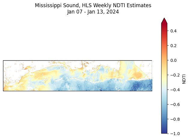
Plotting the results

Once .persist() is called on the DataArray, the Dask computation graph begins to execute and the data is loaded into memory. As such, visualization and further analysis can be performed on the resulting DataArray as usual.

import matplotlib.pyplot as plt
from matplotlib.animation import FuncAnimation
from IPython.display import HTML
from pandas import Timedelta

fig, ax = plt.subplots(figsize=(8, 5))

vmin = -1.0
vmax = 0.5

def update(frame):
    ax.clear()
    weekly_ndti.isel(time=frame).plot.imshow(
        ax=ax, add_colorbar=False, cmap='RdYlBu_r', vmin=vmin, vmax=vmax
    )

    ax.set_title(None)
    ax.set_aspect('equal')
    ax.axis('off')
    x_lim, ylim = ax.get_xlim(), ax.get_ylim()
    ms_sound_gdf.boundary.plot(ax=ax, color='black', linewidth=1)

    ax.set_xlim(x_lim)
    ax.set_ylim(ylim)

    # fig.suptitle(f"Oktibbeha County, MS Sentinel-2 Mean EVI\n" + \
    fig.suptitle(f"Mississippi Sound, HLS Weekly NDTI Estimates\n" + \
        f"{weekly_ndti['time'][frame].dt.strftime('%b %d').values} - " + \
        f"{(weekly_ndti['time'][frame] + Timedelta(days=6)).dt.strftime('%b %d, %Y').values}")

init_plot = weekly_ndti.isel(time=0).plot.imshow(
    ax=ax, add_colorbar=True, cbar_kwargs={'label': 'NDTI'}, cmap='RdYlBu_r', vmin=vmin, vmax=vmax
)

ani = FuncAnimation(fig, update, frames=len(weekly_ndti['time']), repeat=False)

# show in notebook
HTML(ani.to_jshtml(fps=1, default_mode='once'))

/home/dh2306/pcxarray/.venv/lib/python3.12/site-packages/dask/_task_spec.py:763: RuntimeWarning: All-NaN slice encountered
  return self.func(*new_argspec, **kwargs)
/home/dh2306/pcxarray/.venv/lib/python3.12/site-packages/dask/_task_spec.py:763: RuntimeWarning: All-NaN slice encountered
  return self.func(*new_argspec, **kwargs)
/home/dh2306/pcxarray/.venv/lib/python3.12/site-packages/dask/_task_spec.py:763: RuntimeWarning: All-NaN slice encountered
  return self.func(*new_argspec, **kwargs)
/home/dh2306/pcxarray/.venv/lib/python3.12/site-packages/dask/_task_spec.py:763: RuntimeWarning: All-NaN slice encountered
  return self.func(*new_argspec, **kwargs)
/home/dh2306/pcxarray/.venv/lib/python3.12/site-packages/dask/_task_spec.py:763: RuntimeWarning: All-NaN slice encountered
  return self.func(*new_argspec, **kwargs)
/home/dh2306/pcxarray/.venv/lib/python3.12/site-packages/dask/_task_spec.py:763: RuntimeWarning: All-NaN slice encountered
  return self.func(*new_argspec, **kwargs)
/home/dh2306/pcxarray/.venv/lib/python3.12/site-packages/dask/_task_spec.py:763: RuntimeWarning: All-NaN slice encountered
  return self.func(*new_argspec, **kwargs)
/home/dh2306/pcxarray/.venv/lib/python3.12/site-packages/dask/_task_spec.py:763: RuntimeWarning: All-NaN slice encountered
  return self.func(*new_argspec, **kwargs)
/home/dh2306/pcxarray/.venv/lib/python3.12/site-packages/dask/_task_spec.py:763: RuntimeWarning: All-NaN slice encountered
  return self.func(*new_argspec, **kwargs)
/home/dh2306/pcxarray/.venv/lib/python3.12/site-packages/dask/_task_spec.py:763: RuntimeWarning: All-NaN slice encountered
  return self.func(*new_argspec, **kwargs)
/home/dh2306/pcxarray/.venv/lib/python3.12/site-packages/dask/_task_spec.py:763: RuntimeWarning: All-NaN slice encountered
  return self.func(*new_argspec, **kwargs)
/home/dh2306/pcxarray/.venv/lib/python3.12/site-packages/dask/_task_spec.py:763: RuntimeWarning: All-NaN slice encountered
  return self.func(*new_argspec, **kwargs)
/home/dh2306/pcxarray/.venv/lib/python3.12/site-packages/dask/_task_spec.py:763: RuntimeWarning: All-NaN slice encountered
  return self.func(*new_argspec, **kwargs)
/home/dh2306/pcxarray/.venv/lib/python3.12/site-packages/dask/_task_spec.py:763: RuntimeWarning: All-NaN slice encountered
  return self.func(*new_argspec, **kwargs)
/home/dh2306/pcxarray/.venv/lib/python3.12/site-packages/dask/_task_spec.py:763: RuntimeWarning: All-NaN slice encountered
  return self.func(*new_argspec, **kwargs)
/home/dh2306/pcxarray/.venv/lib/python3.12/site-packages/dask/_task_spec.py:763: RuntimeWarning: All-NaN slice encountered
  return self.func(*new_argspec, **kwargs)
/home/dh2306/pcxarray/.venv/lib/python3.12/site-packages/dask/_task_spec.py:763: RuntimeWarning: All-NaN slice encountered
  return self.func(*new_argspec, **kwargs)
/home/dh2306/pcxarray/.venv/lib/python3.12/site-packages/dask/_task_spec.py:763: RuntimeWarning: All-NaN slice encountered
  return self.func(*new_argspec, **kwargs)
/home/dh2306/pcxarray/.venv/lib/python3.12/site-packages/dask/_task_spec.py:763: RuntimeWarning: All-NaN slice encountered
  return self.func(*new_argspec, **kwargs)
/home/dh2306/pcxarray/.venv/lib/python3.12/site-packages/dask/_task_spec.py:763: RuntimeWarning: All-NaN slice encountered
  return self.func(*new_argspec, **kwargs)
/home/dh2306/pcxarray/.venv/lib/python3.12/site-packages/dask/_task_spec.py:763: RuntimeWarning: All-NaN slice encountered
  return self.func(*new_argspec, **kwargs)
/home/dh2306/pcxarray/.venv/lib/python3.12/site-packages/dask/_task_spec.py:763: RuntimeWarning: All-NaN slice encountered
  return self.func(*new_argspec, **kwargs)
/home/dh2306/pcxarray/.venv/lib/python3.12/site-packages/dask/_task_spec.py:763: RuntimeWarning: All-NaN slice encountered
  return self.func(*new_argspec, **kwargs)
/home/dh2306/pcxarray/.venv/lib/python3.12/site-packages/dask/_task_spec.py:763: RuntimeWarning: All-NaN slice encountered
  return self.func(*new_argspec, **kwargs)

Once Loop Reflect